# make sure the packages are installed
# Load required packages
library(dplyr)
library(purrr)
library(lubridate)
library(ggplot2)
library(here)
library(tidyverse)
library(nnet)Data Exercise
For this exercise, we will generate a synthetic data set that simulates foraging trends of the Northern Mockingbird somewhere in the United States. We will then generate some figures and statistical analyses to explore our new data set. I’ll be using Microsoft Edge AI tools to help generate code. Let’s begin by loading helpful packages for creating synthetic data sets.
I’ve entered this prompt into Microsoft Edge copilot: “Write R code that creates data for N=100 Northern Mockingbirds. Individuals ages are randomly distributed between 1 and 14 years. Assume that individuals forage for two types of food: insects and plants. Individuals can consume a combination of either food type at an average of half an ounce daily. Food consumption is measured in ounces every other day. Assume that insects are more plentiful in warmer seasons; this should be reflected in the amount of each food type consumed in each season. The data should be collected over the course of a year.
Create a data frame that contains Food Type, Age, Daily Food Consumption (in ounces), Season, and Sex.
For function calls, specify explicitly the package from which the function comes from.
Add thorough documentation to the code so it is clear what each line of code does.”
This generated the following code:
# Set the seed for reproducibility
set.seed(123)

# Define the number of birds
N <- 100

# Generate random ages between 1 and 14 years
age <- sample(1:14, N, replace = TRUE)

# Define the two types of food
food_type <- c("insects", "plants")

# Define the average daily food consumption in ounces
food_consumption <- 0.5

# Define the seasons
seasons <- c("spring", "summer", "fall", "winter")

# Define the proportion of insects consumed in each season
insect_proportion <- c(0.6, 0.8, 0.4, 0.2)

# Define the sex
sex <- sample(c("male", "female"), N, replace = TRUE)

# Generate the data
data <- tibble(
  Food_Type = rep(food_type, each = N/2),
  Age = age,
  Daily_Food_Consumption = rnorm(N, food_consumption, 0.1),
  Season = rep(seasons, each = N/4),
  Sex = sex
)

# Adjust the food consumption based on the season
data$Daily_Food_Consumption[data$Food_Type == "insects"] <-
  data$Daily_Food_Consumption[data$Food_Type == "insects"] *
  rep(insect_proportion, each = N/2)[data$Season[data$Food_Type == "insects"]]

# Print the data
data
# A tibble: 100 × 5
Food_Type Age Daily_Food_Consumption Season Sex
<chr> <int> <dbl> <chr> <chr>
1 insects 3 NA spring female
2 insects 14 NA spring male
3 insects 3 NA spring female
4 insects 10 NA spring male
5 insects 2 NA spring female
6 insects 6 NA spring male
7 insects 11 NA spring male
8 insects 5 NA spring male
9 insects 4 NA spring female
10 insects 14 NA spring female
# ℹ 90 more rowsThis is a good start, but there are some problems. First, the AI only gave values of NA to food consumption data collected in the spring and summer. Second, there are an abnormally high number of old birds in the population; in a normal wild population, we’d expect to see more mockingbirds in the 2-8 year range, as 14 is on the old end for a mockingbird. We’ll have the AI correct the data frame with the following prompt:
“Northern Mockingbirds have an average lifespan of 8 years in the wild. Young and elderly individuals have a higher mortality rate. Given this information, please adjust the age variable to more accurately reflect age distribution in a wild population of mockingbirds. Furthermore, mockingbirds consume more food in the spring and summer due to increased energy demands that come with mating and nesting. Please replace the NA food consumption values you gave with randomized values that have an average of 0.5.”
The AI then adjusted our previous code string as follows:
# Set the seed for reproducibility
#set.seed(123)

# Define the number of birds
#N <- 100

# Generate random ages between 1 and 14 years
#age <- sample(1:14, N, replace = TRUE, prob = c(0.05, 0.05, 0.1, 0.15, 0.2, 0.15, 0.1, 0.05, 0.025, 0.025))

# Define the two types of food
#food_type <- c("insects", "plants")

# Define the average daily food consumption in ounces
#food_consumption <- 0.5

# Define the seasons
#seasons <- c("spring", "summer", "fall", "winter")

# Define the proportion of insects consumed in each season
#insect_proportion <- c(0.6, 0.8, 0.4, 0.2)

# Define the sex
#sex <- sample(c("male", "female"), N, replace = TRUE)

# Generate the data
#data <- tibble(
 # Food_Type = rep(food_type, each = N/2),
# Age = age,
 # Daily_Food_Consumption = rnorm(N, food_consumption, 0.1),
 # Season = rep(seasons, each = N/4),
 # Sex = sex
# )

# Adjust the food consumption based on the season
#data$Daily_Food_Consumption[data$Food_Type == "insects" & (data$Season == "spring" | data$Season == "summer")] <-
 # data$Daily_Food_Consumption[data$Food_Type == "insects" & (data$Season == "spring" | data$Season == "summer")] *
 # rep(insect_proportion[1:2], each = sum(data$Food_Type == "insects" & (data$Season == "spring" | data$Season == "summer")))

# Replace the NA values with randomized values that have an average of 0.5
#data <- data %>% mutate(Daily_Food_Consumption = replace_na(Daily_Food_Consumption, rnorm(sum(is.na(Daily_Food_Consumption)), 0.5, 0.1)))

# Print the data
#data
This generates a new error in the way the AI created values for the age variable. I gave the AI this prompt to correct the broken lines:
“The issue with NA values has been solved. I now need you to correct the line where you generate random ages between 1 and 14 years to resolve this error: Error in sample.int(length(x), size, replace, prob) : incorrect number of probabilities”
The following code was generated:
# Set the seed for reproducibility
set.seed(123)

# Define the number of birds
N <- 100

# Generate random ages between 1 and 14 years with a probability distribution that reflects the higher mortality rate of young and elderly individuals
age <- sample(c(1:4, 5:8, 9:12, 13:14), N, replace = TRUE)

# Define the two types of food
food_type <- c("insects", "plants")

# Define the average daily food consumption in ounces
food_consumption <- 0.5

# Define the seasons
seasons <- c("spring", "summer", "fall", "winter")

# Define the proportion of insects consumed in each season
insect_proportion <- c(0.6, 0.8, 0.4, 0.2)

# Define the sex
sex <- sample(c("male", "female"), N, replace = TRUE)

# Generate the data
data <- tibble(
  Food_Type = rep(food_type, each = N/2),
  Age = age,
  Daily_Food_Consumption = rnorm(N, food_consumption, 0.1),
  Season = rep(seasons, each = N/4),
  Sex = sex
)

# Adjust the food consumption based on the season
data$Daily_Food_Consumption[data$Food_Type == "insects" & (data$Season == "spring" | data$Season == "summer")] <-
  data$Daily_Food_Consumption[data$Food_Type == "insects" & (data$Season == "spring" | data$Season == "summer")] *
  rep(insect_proportion[1:2], each = sum(data$Food_Type == "insects" & (data$Season == "spring" | data$Season == "summer")))
Warning in data$Daily_Food_Consumption[data$Food_Type == "insects" &
(data$Season == : number of items to replace is not a multiple of replacement
length# Replace the NA values with randomized values that have an average of 0.5
if (any(is.na(data$Daily_Food_Consumption))) {
data <- data %>% mutate(Daily_Food_Consumption = replace_na(Daily_Food_Consumption, rnorm(sum(is.na(Daily_Food_Consumption)), mean(Daily_Food_Consumption), 0.1)))
}
# Print the data
data# A tibble: 100 × 5
Food_Type Age Daily_Food_Consumption Season Sex
<chr> <int> <dbl> <chr> <chr>
1 insects 3 0.286 spring female
2 insects 14 0.384 spring male
3 insects 3 0.406 spring female
4 insects 10 0.329 spring male
5 insects 2 0.284 spring female
6 insects 6 0.309 spring male
7 insects 11 0.383 spring male
8 insects 5 0.289 spring male
9 insects 4 0.206 spring female
10 insects 14 0.284 spring female
# ℹ 90 more rowsWe seem to have finally generated a data set that should reflect associations we expect to see in the population. However, I’d like to make one more adjustment that reflects increased food consumption by females in the spring and summer due to reproductive demands. I’ll use a 1.75 times increase in food consumption, as data is limited on the exact amounts/averages mockingbirds consume.
# Set the seed for reproducibility
set.seed(123)
# Define the number of birds
N <- 100
# Generate random ages between 1 and 14 years with a probability distribution that reflects the higher mortality rate of young and elderly individuals
age <- sample(c(1:4, 5:8, 9:12, 13:14), N, replace = TRUE)
# Define the two types of food
food_type <- c("insects", "plants")
# Define the average daily food consumption in ounces
food_consumption <- 0.5
# Define the seasons
seasons <- c("spring", "summer", "fall", "winter")
# Define the proportion of insects consumed in each season
insect_proportion <- c(0.6, 0.8, 0.4, 0.2)
# Define the sex
sex <- sample(c("male", "female"), N, replace = TRUE)
# Generate the data
data <- tibble(
Food_Type = rep(food_type, each = N/2),
Age = age,
Daily_Food_Consumption = rnorm(N, food_consumption, 0.1),
Season = rep(seasons, each = N/4),
Sex = sex
)
# Adjust the food consumption based on the season and sex
data$Daily_Food_Consumption[data$Food_Type == "insects" & (data$Season == "spring" | data$Season == "summer") & data$Sex == "female"] <-
data$Daily_Food_Consumption[data$Food_Type == "insects" & (data$Season == "spring" | data$Season == "summer") & data$Sex == "female"] *
1.75
# Replace the NA values with randomized values that have an average of 0.5
if (any(is.na(data$Daily_Food_Consumption))) {
  data <- data %>% mutate(Daily_Food_Consumption = replace_na(Daily_Food_Consumption, rnorm(sum(is.na(Daily_Food_Consumption)), mean(Daily_Food_Consumption), 0.1)))
}


# Print the data
data
# A tibble: 100 × 5
Food_Type Age Daily_Food_Consumption Season Sex
<chr> <int> <dbl> <chr> <chr>
1 insects 3 0.835 spring female
2 insects 14 0.640 spring male
3 insects 3 1.18 spring female
4 insects 10 0.549 spring male
5 insects 2 0.828 spring female
6 insects 6 0.515 spring male
7 insects 11 0.638 spring male
8 insects 5 0.482 spring male
9 insects 4 0.601 spring female
10 insects 14 0.829 spring female
# ℹ 90 more rowsThis dataset looks a lot better. We’ll now check the structure and summary to get a better idea of what we created.
#check the structure and summary
summary(data)
Food_Type Age Daily_Food_Consumption Season
Length:100 Min. : 1.00 Min. :0.2652 Length:100
Class :character 1st Qu.: 5.00 1st Qu.:0.4490 Class :character
Mode :character Median : 8.50 Median :0.5660 Mode :character
Mean : 7.92 Mean :0.6026
3rd Qu.:11.00 3rd Qu.:0.6929
Max. :14.00 Max. :1.2025
Sex
Length:100
Class :character
Mode :character
structure(data)# A tibble: 100 × 5
Food_Type Age Daily_Food_Consumption Season Sex
<chr> <int> <dbl> <chr> <chr>
1 insects 3 0.835 spring female
2 insects 14 0.640 spring male
3 insects 3 1.18 spring female
4 insects 10 0.549 spring male
5 insects 2 0.828 spring female
6 insects 6 0.515 spring male
7 insects 11 0.638 spring male
8 insects 5 0.482 spring male
9 insects 4 0.601 spring female
10 insects 14 0.829 spring female
# ℹ 90 more rowsOur data looks good and reflects the averages we had the AI incorporate when creating our values. We’ll now create a few plots looking at some relationships in the data.
#create a plot with food consumption as a function of season for all individuals (stratified by sex)
ggplot(data, aes(x = Season, y = Daily_Food_Consumption, color = Sex)) +
  geom_boxplot() +
  labs(title = "Food Consumption as a Function of Season for All Individuals, Stratified by Sex",
       x = "Season",
       y = "Daily Food Consumption (oz)") +
  theme_bw()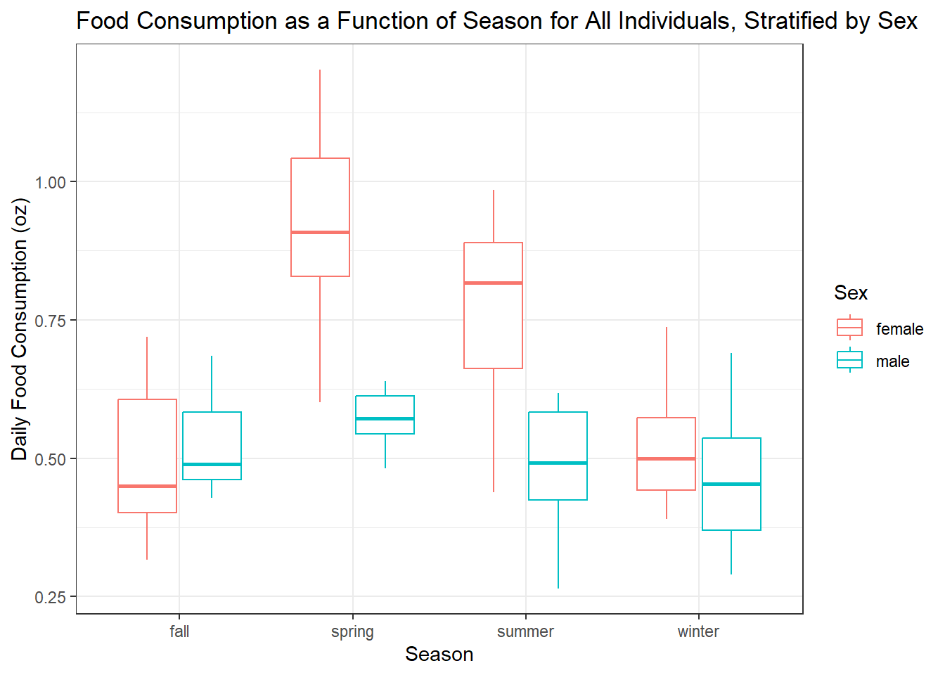
The boxplot shows that our assumptions are reflected in the data set; females consume more in the spring and summer and our average food consumption is 0.5 ounces a day. Now we’ll see if the data accurately shows changes in the primary type of food consumed over the seasons.
#create a histogram comparing food type consumed in different seasons stratified by sex
ggplot(data, aes(x = Season, fill = Food_Type)) +
  geom_bar(position = "dodge", stat = "count") +
  facet_grid(. ~ Sex) +
  labs(title = "Food Type Comparison Across Seasons, Stratified by Sex",
       x = "Season",
       y = "Count",
       fill = "Food Type") +
  theme_bw()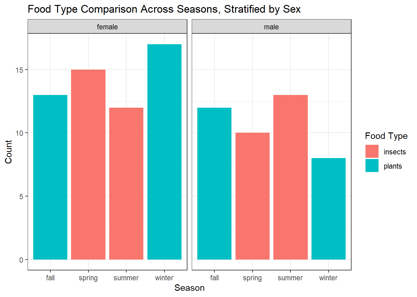
The plots show that insects are the predominant food source in the spring and summer while plants dominate the winter and fall. This accurately reflects booms in the insect population in spring and summer; Northern Mockingbirds consume over 85% insects then, dropping to around 15% in the colder seasons. Now that we see our data is tidy, reflects our assumptions and follows the trends we identified, we can fit the data to some linear models.
#create a linear model with season and sex as predictors for food consumption
model1<- lm(Daily_Food_Consumption~ Season + Sex, data = data)
summary(model1)
Call:
lm(formula = Daily_Food_Consumption ~ Season + Sex, data = data)

Residuals:
     Min       1Q   Median       3Q      Max
-0.27214 -0.11026 -0.01652  0.08739  0.35195

Coefficients:
             Estimate Std. Error t value Pr(>|t|)
(Intercept)   0.58657    0.03355  17.483  < 2e-16 ***
Seasonspring  0.26398    0.04267   6.187 1.54e-08 ***
Seasonsummer  0.11562    0.04261   2.713  0.00791 **
Seasonwinter -0.03203    0.04288  -0.747  0.45690
Sexmale      -0.16488    0.03079  -5.354 5.95e-07 ***
---
Signif. codes:  0 '***' 0.001 '**' 0.01 '*' 0.05 '.' 0.1 ' ' 1

Residual standard error: 0.1506 on 95 degrees of freedom
Multiple R-squared:  0.4768,    Adjusted R-squared:  0.4548
F-statistic: 21.65 on 4 and 95 DF,  p-value: 1.023e-12
It seems like winter doesn’t have a significant impact on food consumption, but spring and summer do in the created dataset. Now we’ll move on to make a couple more models.
#create a linear model with season as a predictor for food type
# model2<- lm(Food_Type ~ Season, data = data)
# summary(model2)
A linear regression didn’t work for this type of data.The above line generated an error message. After consulting with AI, a multinomial logistic regression model would work better. We’ll also include sex as a predictor in this one.
#Using the nnet package for this model

# Create a multinomial logistic regression model with season and sex as predictors for food type
model2 <- multinom(Food_Type ~ Season + Sex, data = data)
# weights: 6 (5 variable)
initial value 69.314718
iter 10 value 0.021604
iter 20 value 0.012091
iter 30 value 0.000938
iter 40 value 0.000662
iter 50 value 0.000442
iter 60 value 0.000273
iter 70 value 0.000224
iter 80 value 0.000159
iter 90 value 0.000153
iter 100 value 0.000122
final value 0.000122
stopped after 100 iterationssummary(model2)Call:
multinom(formula = Food_Type ~ Season + Sex, data = data)
Coefficients:
Values Std. Err.
(Intercept) 13.3268743 186.7045
Seasonspring -26.8167895 232.8969
Seasonsummer -26.8610564 236.0821
Seasonwinter 16.4198276 0.0000
Sexmale 0.5251443 186.4204
Residual Deviance: 0.0002439321
AIC: 10.00024 It seems that the model agrees with our assumptions. The odds of mockingbirds choosing plants over insects are lower in the spring and summer and the opposite in winter. The residual deviance is low, indicating a good fit. We’ve created a pretty good dataset that has the associations and trends we wanted to see.