#Load packages
library(tidymodels)
library(ggplot2)
library(here)
library(dplyr)
library(corrplot)
library(glmnet)
library(ranger)
library(tune)
library(dials)
#Load the data
mldata<- readRDS(here("ml-models-exercise", "modelfitting.rds"))

#seed setting
rngseed=1234ml-models-exercise
For this exercise, we’ll be practicing some machine learning models using the data from our previous “Fitting exercise”. Much of the base code for this exercise was generated using Microsoft Copilot in Precise Mode; this was then modified to the specifics of our data and to fix errors. We’ll start by loading packages, the data, and creating a random seed for reproducibility.
Now we’ll do some data processing. We’ll combine the “7” and “88” categories for our RACE variable into a new category, “3”.
# Change 7 and 88 to 3.
# Convert RACE to numeric
mldata$RACE <- as.numeric(as.character(mldata$RACE))

# Perform the replacement
mldata <- mldata %>%
  mutate(RACE = case_when(
    RACE %in% c(7, 88) ~ 3,
    TRUE ~ RACE
  ))

# Convert RACE back to factor
mldata$RACE <- as.factor(mldata$RACE)

#Double check to make sure everything is the class we want it
class(mldata$RACE)
[1] "factor"Now we’ll make a pairwise correlation plot for our continuous variables to make sure we don’t have too much collinearity between variables.
# Select the variables
continuous_vars <- mldata[, c("Y", "DOSE", "AGE", "WT", "HT")]

# Compute correlation matrix
correlation_matrix <- cor(continuous_vars)

# Create a pairwise correlation plot (using corrplot)
corrplot(correlation_matrix, method = "circle")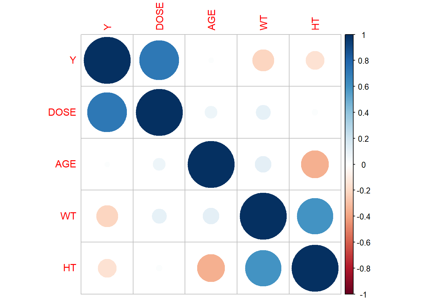
Nothing seems to correlated (absolute value of 0.9+), so we can continue with our modelling. We’ll first create a new variable for Body Mass Index (BMI) using the values in our HT and WT columns.
# Compute BMI from our height and weight data (assumed to be in meters and kg. based off of the values)
mldata$BMI <- mldata$WT / (mldata$HT^2)
With all of our cleaning done, we can now proceed to fitting. We’ll do 3 models: a GLM with all predictors, a LASSO model, and a random forest model. We’ll use the tidymodels framework for all of these.
# Set seed for reproducibility
set.seed(rngseed)

# Define the outcome and predictors
outcome <- "Y"
predictors <- setdiff(names(mldata), outcome)

# Create a recipe
recipe <- recipe(formula = Y ~ ., data = mldata) %>%
  step_dummy(all_nominal(), -all_outcomes()) %>%
  step_normalize(all_predictors())

# Define the models
# 1. Linear Model
all_model <- linear_reg() %>%
  set_engine("lm") %>%
  set_mode("regression")

# 2. LASSO Model
lasso_model <- linear_reg(penalty = 0.1, mixture = 1) %>%
  set_engine("glmnet") %>%
  set_mode("regression")

# 3. Random Forest Model
rf_model <- rand_forest() %>%
  set_engine("ranger", seed = rngseed) %>%
  set_mode("regression")

# Create workflows
all_workflow <- workflow() %>%
  add_model(all_model) %>%
  add_recipe(recipe)

lasso_workflow <- workflow() %>%
  add_model(lasso_model) %>%
  add_recipe(recipe)

rf_workflow <- workflow() %>%
  add_model(rf_model) %>%
  add_recipe(recipe)

# Fit the models
all_fit <- all_workflow %>%
  fit(data = mldata)

lasso_fit <- lasso_workflow %>%
  fit(data = mldata)

rf_fit <- rf_workflow %>%
  fit(data = mldata)
Now that we’ve fit the models, we can begin to evaluate their performance. We’ll use RMSE as the metric and create some plots.
# Make predictions
all_preds <- predict(all_fit, new_data = mldata)
lasso_preds <- predict(lasso_fit, new_data = mldata)
rf_preds <- predict(rf_fit, new_data = mldata)

# Calculate RMSE
#augment to evaluate performance metric
aug_all<- augment(all_fit, mldata)
aug_all %>% select(Y, .pred)
# A tibble: 120 × 2
Y .pred
<dbl> <dbl>
1 2691. 1666.
2 2639. 1951.
3 2150. 1896.
4 1789. 1548.
5 3126. 2369.
6 2337. 1921.
7 3007. 1510.
8 2796. 2156.
9 3866. 2658.
10 1762. 1352.
# ℹ 110 more rows#LASSO augment
aug_lasso<- augment(lasso_fit, mldata)
aug_lasso %>% select(Y, .pred)# A tibble: 120 × 2
Y .pred
<dbl> <dbl>
1 2691. 1665.
2 2639. 1951.
3 2150. 1901.
4 1789. 1553.
5 3126. 2358.
6 2337. 1929.
7 3007. 1513.
8 2796. 2154.
9 3866. 2644.
10 1762. 1345.
# ℹ 110 more rows#Forest augment
aug_rf<- augment(rf_fit, mldata)
aug_rf %>% select(Y, .pred)# A tibble: 120 × 2
Y .pred
<dbl> <dbl>
1 2691. 2229.
2 2639. 2379.
3 2150. 1934.
4 1789. 1818.
5 3126. 2740.
6 2337. 1977.
7 3007. 2277.
8 2796. 2518.
9 3866. 2959.
10 1762. 1617.
# ℹ 110 more rows#get RMSE of models
all_rmse<- aug_all %>% rmse(truth = Y, .pred)
lasso_rmse <- aug_lasso %>% rmse(truth = Y, .pred)
rf_rmse <- aug_rf %>% rmse(truth = Y, .pred)
# Print RMSE
print(paste("Linear Model RMSE: ", all_rmse))[1] "Linear Model RMSE: rmse"
[2] "Linear Model RMSE: standard"
[3] "Linear Model RMSE: 571.595397430179"print(paste("LASSO Model RMSE: ", lasso_rmse))[1] "LASSO Model RMSE: rmse" "LASSO Model RMSE: standard"
[3] "LASSO Model RMSE: 571.650382196397"print(paste("Random Forest Model RMSE: ", rf_rmse))[1] "Random Forest Model RMSE: rmse"
[2] "Random Forest Model RMSE: standard"
[3] "Random Forest Model RMSE: 381.596767379991"# Create observed vs predicted plots
ggplot() +
geom_point(aes(x = mldata$Y, y = all_preds$.pred), color = "blue") +
geom_abline(intercept = 0, slope = 1, color = "red") +
ggtitle("Linear Model: Observed vs Predicted") +
xlab("Observed") +
ylab("Predicted")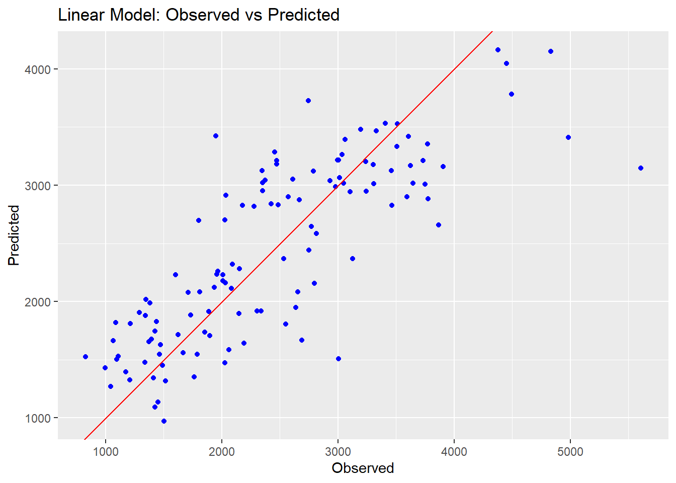
ggplot() +
  geom_point(aes(x = mldata$Y, y = lasso_preds$.pred), color = "blue") +
  geom_abline(intercept = 0, slope = 1, color = "red") +
  ggtitle("LASSO Model: Observed vs Predicted") +
  xlab("Observed") +
  ylab("Predicted")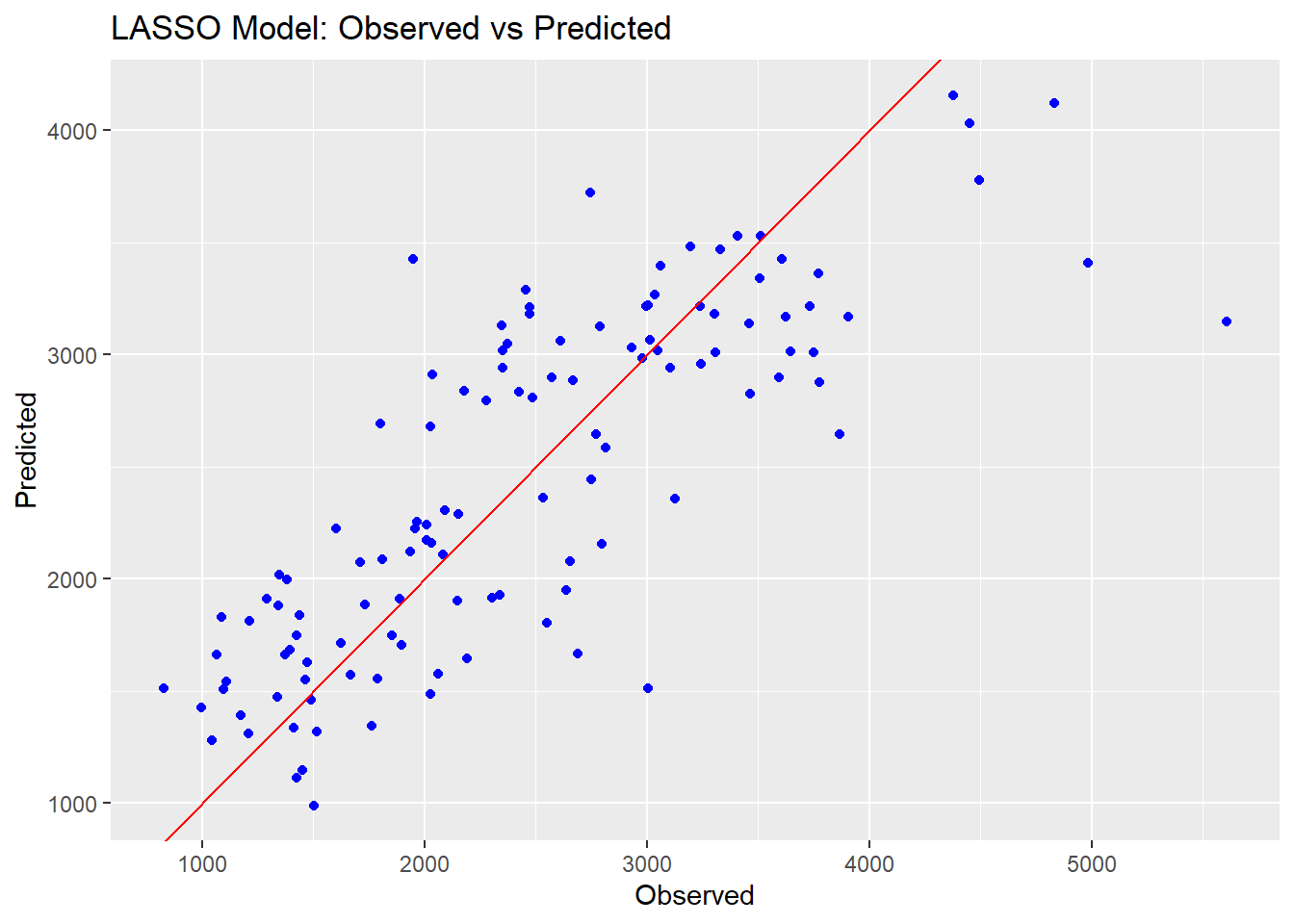
ggplot() +
  geom_point(aes(x = mldata$Y, y = rf_preds$.pred), color = "blue") +
  geom_abline(intercept = 0, slope = 1, color = "red") +
  ggtitle("Random Forest Model: Observed vs Predicted") +
  xlab("Observed") +
  ylab("Predicted")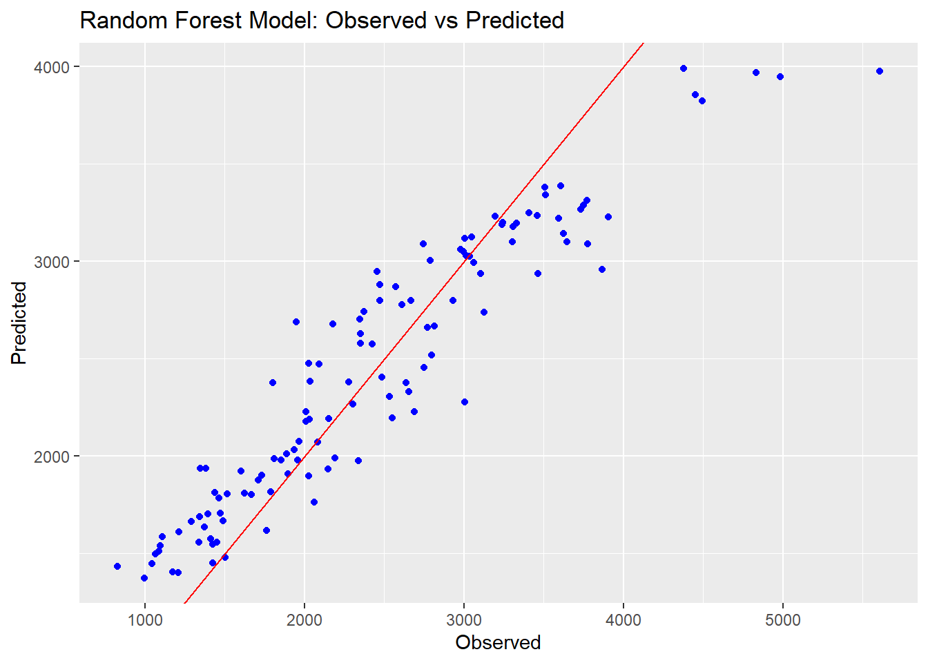
We can see that the Random Forest model performs a lot better on the RMSE metric than the other two models. The prediction points are also closer to the line on the observed vs predicted plots, indicating a better fit overall. The linear and LASSO models are very similar to each other; this is likely because we set the tuning paramter so low for our LASSO, resulting in very little change from a typical linear model.
We’ll now practice tuning our complex models (LASSO and RF). We’ll start with LASSO. Note that this tuning is being done with the data used to train the model; this is a poor choice in a real analysis and is only being done now for practice purposes.
# Define the grid of parameters
penalty_values <- 10^seq(-5, 2, length.out = 50)
penalty_grid <- tibble(penalty = penalty_values)

# Update the LASSO model specification to include the penalty parameter
lasso_model <- linear_reg(penalty = tune(), mixture = 1) %>%
  set_engine("glmnet") %>%
  set_mode("regression")

# Update the LASSO workflow to include the updated model specification
lasso_workflow <- workflow() %>%
  add_model(lasso_model) %>%
  add_recipe(recipe)

# Create resamples using the apparent() function
resamples <- apparent(mldata)

# Tune the LASSO model
tune_results <- tune_grid(
  lasso_workflow,
  resamples = resamples,
  grid = penalty_grid
)

# Print the tuning results
print(tune_results)
# Tuning results
# Apparent sampling
# A tibble: 1 × 4
splits id .metrics .notes
<list> <chr> <list> <list>
1 <split [120/120]> Apparent <tibble [100 × 5]> <tibble [0 × 3]># Plot the tuning results
autoplot(tune_results)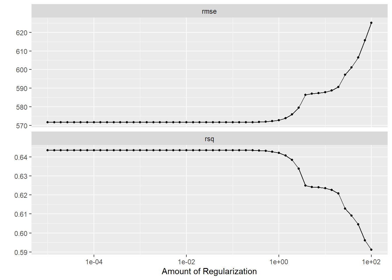
We can see that as our penalty parameter increases, the RMSE in our LASSO model also increases. Low penalty values hover at the same RMSE as our linear model; this could indicate that we have no overfitting in our model or that all predictors are relevant. However, we know that we’re tuning our model with the same data we used to fit it, so these results are misleading since we aren’t actually able to test our model with new data. Now we’ll tune our RF model.
# Update the Random Forest model specification to include the mtry and min_n parameters
rf_model <- rand_forest(mtry = tune(), min_n = tune(), trees = 300) %>%
  set_engine("ranger", seed = rngseed) %>%
  set_mode("regression")

# Update the Random Forest workflow to include the updated model specification
rf_workflow <- workflow() %>%
  add_model(rf_model) %>%
  add_recipe(recipe)

# Define the grid of parameters
mtry_param <- mtry(range = c(1, 7))
min_n_param <- min_n(range = c(1, 21))
rf_grid <- grid_regular(mtry_param, min_n_param, levels = 7)

# Tune the Random Forest model
tune_results <- tune_grid(
  rf_workflow,
  resamples = resamples,
  grid = rf_grid
)

# Print the tuning results
print(tune_results)
# Tuning results
# Apparent sampling
# A tibble: 1 × 4
splits id .metrics .notes
<list> <chr> <list> <list>
1 <split [120/120]> Apparent <tibble [98 × 6]> <tibble [0 × 3]># Plot the tuning results
autoplot(tune_results)
It seems that a higher value of mtry and a lower value of min_n lead to the best results. We’ll move on for now to using CV then actually tuning the data to “new” observations.
#set the seed again
set.seed(rngseed)

# Create real resamples using 5-fold cross-validation, 5 times repeated
resamples <- vfold_cv(mldata, v = 5, repeats = 5)

# Define the grid of parameters for LASSO
penalty_values <- 10^seq(-5, 2, length.out = 50)
penalty_grid <- tibble(penalty = penalty_values)

# Tune the LASSO model
tune_results_lasso <- tune_grid(
  lasso_workflow,
  resamples = resamples,
  grid = penalty_grid
)

# Print the tuning results for LASSO
print(tune_results_lasso)
# Tuning results
# 5-fold cross-validation repeated 5 times
# A tibble: 25 × 5
splits id id2 .metrics .notes
<list> <chr> <chr> <list> <list>
1 <split [96/24]> Repeat1 Fold1 <tibble [100 × 5]> <tibble [0 × 3]>
2 <split [96/24]> Repeat1 Fold2 <tibble [100 × 5]> <tibble [0 × 3]>
3 <split [96/24]> Repeat1 Fold3 <tibble [100 × 5]> <tibble [0 × 3]>
4 <split [96/24]> Repeat1 Fold4 <tibble [100 × 5]> <tibble [0 × 3]>
5 <split [96/24]> Repeat1 Fold5 <tibble [100 × 5]> <tibble [0 × 3]>
6 <split [96/24]> Repeat2 Fold1 <tibble [100 × 5]> <tibble [0 × 3]>
7 <split [96/24]> Repeat2 Fold2 <tibble [100 × 5]> <tibble [0 × 3]>
8 <split [96/24]> Repeat2 Fold3 <tibble [100 × 5]> <tibble [0 × 3]>
9 <split [96/24]> Repeat2 Fold4 <tibble [100 × 5]> <tibble [0 × 3]>
10 <split [96/24]> Repeat2 Fold5 <tibble [100 × 5]> <tibble [0 × 3]>
# ℹ 15 more rows# Plot the tuning results for LASSO
autoplot(tune_results_lasso)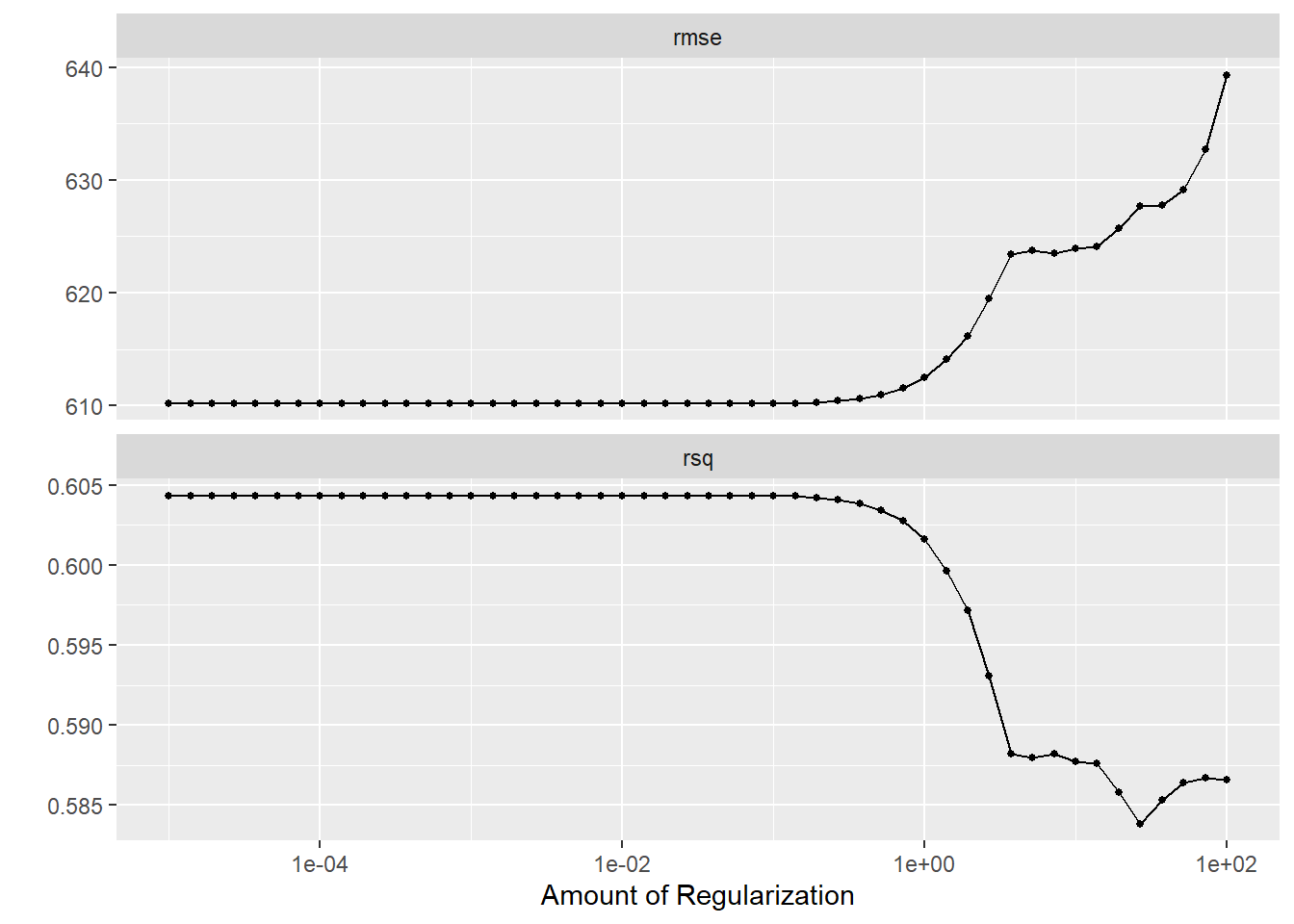
# Define the grid of parameters for Random Forest
rf_param_grid <- grid_regular(
  mtry(range = c(1, 7)),
  min_n(range = c(1, 21)),
  levels = 7
)

# Tune the Random Forest model
tune_results_rf <- tune_grid(
  rf_workflow,
  resamples = resamples,
  grid = rf_param_grid
)

# Print the tuning results for Random Forest
print(tune_results_rf)
# Tuning results
# 5-fold cross-validation repeated 5 times
# A tibble: 25 × 5
splits id id2 .metrics .notes
<list> <chr> <chr> <list> <list>
1 <split [96/24]> Repeat1 Fold1 <tibble [98 × 6]> <tibble [0 × 3]>
2 <split [96/24]> Repeat1 Fold2 <tibble [98 × 6]> <tibble [0 × 3]>
3 <split [96/24]> Repeat1 Fold3 <tibble [98 × 6]> <tibble [0 × 3]>
4 <split [96/24]> Repeat1 Fold4 <tibble [98 × 6]> <tibble [0 × 3]>
5 <split [96/24]> Repeat1 Fold5 <tibble [98 × 6]> <tibble [0 × 3]>
6 <split [96/24]> Repeat2 Fold1 <tibble [98 × 6]> <tibble [0 × 3]>
7 <split [96/24]> Repeat2 Fold2 <tibble [98 × 6]> <tibble [0 × 3]>
8 <split [96/24]> Repeat2 Fold3 <tibble [98 × 6]> <tibble [0 × 3]>
9 <split [96/24]> Repeat2 Fold4 <tibble [98 × 6]> <tibble [0 × 3]>
10 <split [96/24]> Repeat2 Fold5 <tibble [98 × 6]> <tibble [0 × 3]>
# ℹ 15 more rows# Plot the tuning results for Random Forest
autoplot(tune_results_rf)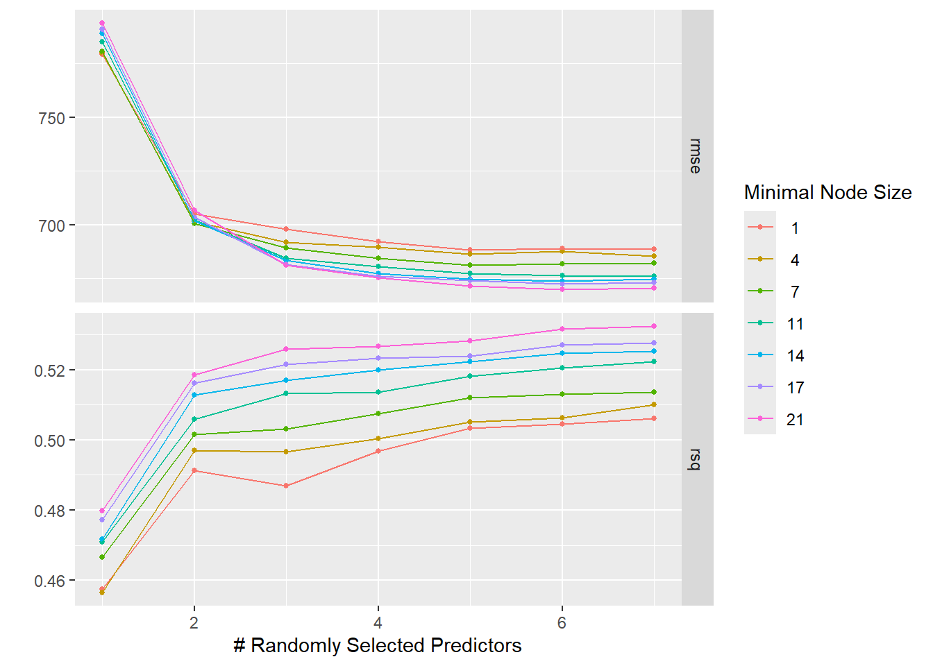
The LASSO still does best for a small penalty, the RMSE for both models went up, and the LASSO now has lower RMSE compared to the RF. CV provides a more robust estimate of model performance by averaging the performance across multiple folds. This often results in a higher RMSE compared to a single model fit on the entire dataset. This could explain why the RMSE for both models went up when using CV. When the penalty is small, LASSO includes more features in the model, making it more flexible and potentially leading to lower RMSE. This could explain why LASSO still does best for a small penalty. LASSO is a linear model, which may be less complex than a Random Forest depending on the number of features selected. If the true relationship is linear/nearly linear, LASSO may outperform a Random Forest, which could explain why LASSO now has a lower RMSE compared to the Random Forest. Based off of these findings, it would seem that the LASSO model explains more variation (higher R squared value) and has a lower RMSE, indicating better performance. I would select this as the better model for our study.